Examples

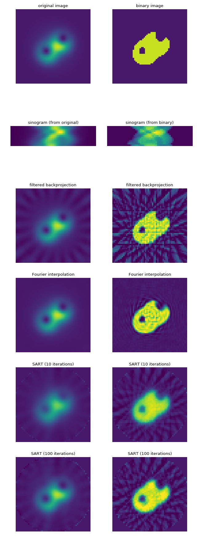
Comparison of parallel-beam reconstruction methods

This example illustrates the performance of the different reconstruction techniques for a parallel-beam geometry. The left column shows the reconstruction of the original image and the right column shows the reconstruction of the corresponding binary images. Note that the SART process could be sped-up by computing an initial guess with a non-iterative method and setting it with the initial keyword argument.

comparison_parallel.py

from matplotlib import pylab as plt
import numpy as np

import radontea
from radontea.logo import get_original

N = 55  # image size
A = 13  # number of sinogram angles
ITA = 10  # number of iterations a
ITB = 100  # number of iterations b

angles = np.linspace(0, np.pi, A)

im = get_original(N)
sino = radontea.radon_parallel(im, angles)
fbp = radontea.backproject(sino, angles)
fintp = radontea.fourier_map(sino, angles).real
sarta = radontea.sart(sino, angles, iterations=ITA)
sartb = radontea.sart(sino, angles, iterations=ITB)

im2 = (im >= (im.max() / 5)) * 255
sino2 = radontea.radon_parallel(im2, angles)
fbp2 = radontea.backproject(sino2, angles)
fintp2 = radontea.fourier_map(sino2, angles).real
sarta2 = radontea.sart(sino2, angles, iterations=ITA)
sartb2 = radontea.sart(sino2, angles, iterations=ITB)

plt.figure(figsize=(8, 22))
pltkw = {"vmin": -20,
         "vmax": 280}

plt.subplot(6, 2, 1, title="original image")
plt.imshow(im, **pltkw)
plt.axis('off')

plt.subplot(6, 2, 2, title="binary image")
plt.imshow(im2, **pltkw)
plt.axis('off')

plt.subplot(6, 2, 3, title="sinogram (from original)")
plt.imshow(sino)
plt.axis('off')

plt.subplot(6, 2, 4, title="sinogram (from binary)")
plt.imshow(sino2)
plt.axis('off')

plt.subplot(6, 2, 5, title="filtered backprojection")
plt.imshow(fbp, **pltkw)
plt.axis('off')

plt.subplot(6, 2, 6, title="filtered backprojection")
plt.imshow(fbp2, **pltkw)
plt.axis('off')

plt.subplot(6, 2, 7, title="Fourier interpolation")
plt.imshow(fintp, **pltkw)
plt.axis('off')

plt.subplot(6, 2, 8, title="Fourier interpolation")
plt.imshow(fintp2, **pltkw)
plt.axis('off')

plt.subplot(6, 2, 9, title="SART ({} iterations)".format(ITA))
plt.imshow(sarta, **pltkw)
plt.axis('off')

plt.subplot(6, 2, 10, title="SART ({} iterations)".format(ITA))
plt.imshow(sarta2, **pltkw)
plt.axis('off')

plt.subplot(6, 2, 11, title="SART ({} iterations)".format(ITB))
plt.imshow(sartb, **pltkw)
plt.axis('off')

plt.subplot(6, 2, 12, title="SART ({} iterations)".format(ITB))
plt.imshow(sartb2, **pltkw)
plt.axis('off')


plt.tight_layout()
plt.show()

Volumetric data reconstruction benchmark

This simple example can be used to quantify the speed-up due to multiprocessing on the hardware used. Note that multiprocessing.cpu_count does not return the number of physical cores.

benchmark_3d.py

from multiprocessing import cpu_count
import time

import numpy as np

import radontea as rt


A = 70    # number of angles
N = 128   # detector size x
M = 24    # detector size y (number of slices)

# generate random data
sino0 = np.random.random((A, N))     # for 2d example
sino = np.random.random((A, M, N))    # for 3d example
sino[:, 0, :] = sino0
angles = np.linspace(0, np.pi, A)     # for both

a = time.time()
data1 = rt.backproject_3d(sino, angles, ncpus=1)
print("time on 1 core:  {:.2f} s".format(time.time() - a))

a = time.time()
data2 = rt.backproject_3d(sino, angles, ncpus=cpu_count())
print("time on {} cores: {:.2f} s".format(cpu_count(), time.time() - a))

assert np.all(data1 == data2), "2D and 3D results don't match"

Progress monitoring with progression

The progress of the reconstruction algorithms in radontea can be tracked with other packages such as progression.

progression_3d.py

from multiprocessing import cpu_count

import numpy as np
import progression as pr

import radontea as rt


A = 55    # number of angles
N = 128   # detector size x
M = 24    # detector size y (number of slices)

# generate random data
sino0 = np.random.random((A, N))
sino = np.random.random((A, M, N))
sino[:, 0, :] = sino0
angles = np.linspace(0, np.pi, A)

count = pr.UnsignedIntValue()
max_count = pr.UnsignedIntValue()


with pr.ProgressBar(count=count,
                    max_count=max_count,
                    interval=0.3
                    ) as pb:
    pb.start()
    rt.volume_recon(func2d=rt.sart, sinogram=sino, angles=angles,
                    ncpus=cpu_count(), count=count, max_count=max_count)